實驗 A 抓收盤價

目錄

• 資料載入
• Pytorch
• PatchTST
• chronos
• TimeFM
• 轉回真實股價
• 畫圖

資料載入

import yfinance as yf
import pandas as pd
import numpy as np
import matplotlib.pyplot as plt


ticker = "AAPL"


data = yf.download(
    ticker,
    start="2010-01-01",
    end="2026-01-01"
)


df = data[["Close"]].copy()


# yfinance 新版可能是 multi-index
if isinstance(df.columns, pd.MultiIndex):
    df.columns = df.columns.get_level_values(0)


df = df.reset_index()


df.columns = [
    "ds",
    "y"
]


df.head()

[*********************100%***********************]  1 of 1 completed

	ds	y
0	2010-01-04	6.406482
1	2010-01-05	6.417558
2	2010-01-06	6.315476
3	2010-01-07	6.303802
4	2010-01-08	6.345711

split = int(len(df)*0.8)


train = df.iloc[:split].copy()

test = df.iloc[split:].copy()


print(train.shape)
print(test.shape)

(3219, 2)
(805, 2)

from sklearn.preprocessing import StandardScaler


scaler = StandardScaler()


train["y_scaled"] = scaler.fit_transform(
    train[["y"]]
)


test["y_scaled"] = scaler.transform(
    test[["y"]]
)


train.head()

	ds	y	y_scaled
0	2010-01-04	6.406482	-0.887651
1	2010-01-05	6.417558	-0.887409
2	2010-01-06	6.315476	-0.889634
3	2010-01-07	6.303802	-0.889889
4	2010-01-08	6.345711	-0.888975

Pytorch

lookback = 120
forecast_horizon = 15


def create_dataset(data, lookback, horizon):

    X = []
    y = []

    values = data["y_scaled"].values

    for i in range(
        len(values) - lookback - horizon + 1
    ):

        # 過去120天
        X.append(
            values[i:i+lookback]
        )

        # 未來15天
        y.append(
            values[i+lookback:i+lookback+horizon]
        )

    return np.array(X), np.array(y)


X_train, y_train = create_dataset(
    train,
    lookback,
    forecast_horizon
)


X_test, y_test = create_dataset(
    test,
    lookback,
    forecast_horizon
)


print(X_train.shape)
print(y_train.shape)

(3085, 120)
(3085, 15)

import torch
import torch.nn as nn


class StockTransformer(nn.Module):

    def __init__(
        self,
        d_model=64,
        nhead=4,
        layers=3,
        horizon=15
    ):
        super().__init__()

        self.input_layer = nn.Linear(
            1,
            d_model
        )

        encoder_layer = nn.TransformerEncoderLayer(
            d_model=d_model,
            nhead=nhead,
            batch_first=True
        )

        self.transformer = nn.TransformerEncoder(
            encoder_layer,
            num_layers=layers
        )

        self.fc = nn.Linear(
            d_model,
            horizon
        )


    def forward(self,x):

        x = self.input_layer(x)

        x = self.transformer(x)

        x = x[:, -1, :]

        x = self.fc(x)

        return x

X_train = torch.tensor(
    X_train,
    dtype=torch.float32
)

y_train = torch.tensor(
    y_train,
    dtype=torch.float32
).reshape(-1,1)

model = StockTransformer()

print(model)

loss_fn = nn.MSELoss()

optimizer = torch.optim.Adam(
    model.parameters(),
    lr=0.001
)

StockTransformer(
  (input_layer): Linear(in_features=1, out_features=64, bias=True)
  (transformer): TransformerEncoder(
    (layers): ModuleList(
      (0-2): 3 x TransformerEncoderLayer(
        (self_attn): MultiheadAttention(
          (out_proj): NonDynamicallyQuantizableLinear(in_features=64, out_features=64, bias=True)
        )
        (linear1): Linear(in_features=64, out_features=2048, bias=True)
        (dropout): Dropout(p=0.1, inplace=False)
        (linear2): Linear(in_features=2048, out_features=64, bias=True)
        (norm1): LayerNorm((64,), eps=1e-05, elementwise_affine=True)
        (norm2): LayerNorm((64,), eps=1e-05, elementwise_affine=True)
        (dropout1): Dropout(p=0.1, inplace=False)
        (dropout2): Dropout(p=0.1, inplace=False)
      )
    )
  )
  (fc): Linear(in_features=64, out_features=15, bias=True)
)

X_test = torch.tensor(
    X_test,
    dtype=torch.float32
)

X_test = X_test.unsqueeze(-1)
print(X_test.shape)

torch.Size([671, 120, 1])

model.eval()

with torch.no_grad():
    stock_pred = model(X_test)

print(stock_pred.shape)

torch.Size([671, 15])

stock_pred = model(X_test)

# 換成真實價格

stock_pred_price = scaler.inverse_transform(
    stock_pred.detach().numpy()
)

stock_pred_price = stock_pred_price[0]

PatchTST

from neuralforecast import NeuralForecast
from neuralforecast.models import PatchTST


nf_train = train[[
    "ds",
    "y_scaled"
]].copy()


nf_train.columns = [
    "ds",
    "y"
]


nf_train["unique_id"] = "AAPL"


model = PatchTST(
    h=15,
    input_size=120,
    patch_len=12,
    stride=6,
    max_steps=300
)


nf = NeuralForecast(
    models=[model],
    freq="D"
)


nf.fit(
    nf_train
)

Seed set to 1
GPU available: True (cuda), used: True
TPU available: False, using: 0 TPU cores
HPU available: False, using: 0 HPUs
You are using a CUDA device ('NVIDIA GeForce RTX 4090') that has Tensor Cores. To properly utilize them, you should set `torch.set_float32_matmul_precision('medium' | 'high')` which will trade-off precision for performance. For more details, read https://pytorch.org/docs/stable/generated/torch.set_float32_matmul_precision.html#torch.set_float32_matmul_precision
LOCAL_RANK: 0 - CUDA_VISIBLE_DEVICES: [0]

  | Name         | Type              | Params | Mode 
-----------------------------------------------------------
0 | loss         | MAE               | 0      | train
1 | padder_train | ConstantPad1d     | 0      | train
2 | scaler       | TemporalNorm      | 0      | train
3 | model        | PatchTST_backbone | 440 K  | train
-----------------------------------------------------------
440 K     Trainable params
3         Non-trainable params
440 K     Total params
1.760     Total estimated model params size (MB)
90        Modules in train mode
0         Modules in eval mode

`Trainer.fit` stopped: `max_steps=300` reached.

patch_forecast = nf.predict()

patch_pred_scaled = (
    patch_forecast["PatchTST"]
    .values)


print(patch_pred_scaled)

GPU available: True (cuda), used: True
TPU available: False, using: 0 TPU cores
HPU available: False, using: 0 HPUs
LOCAL_RANK: 0 - CUDA_VISIBLE_DEVICES: [0]

[1.9465663 1.9714975 1.9953431 2.0224025 2.0214329 2.0373554 2.0497112
 2.0394096 2.0960329 2.0887506 2.1207821 2.0824437 2.0865793 2.1142323
 2.039461 ]

chronos

import torch
from chronos import ChronosPipeline


context = torch.tensor(
    train["y_scaled"].values,
    dtype=torch.float32
)


pipeline = ChronosPipeline.from_pretrained(
    "amazon/chronos-t5-small",
    device_map="auto"
)


forecast = pipeline.predict(
    context,
    prediction_length=15
)


print(forecast.shape)

torch.Size([1, 20, 15])

chronos_pred_scaled = (
    forecast
    .mean(dim=1)
    .squeeze()
    .numpy()
)


print(chronos_pred_scaled)

[1.9613361 1.9613361 1.955292  1.9620917 1.9477367 1.9326261 1.9401814
 1.9333817 1.951514  1.9515142 1.9711578 1.9756911 1.9764465 1.9794686
 1.9749353]

TimeFM

import timesfm
import numpy as np


timesfm_model = timesfm.TimesFM_2p5_200M_torch.from_pretrained(
    "google/timesfm-2.5-200m-pytorch"
)


timesfm_model.compile(
    timesfm.ForecastConfig(
        max_context=512,
        max_horizon=128
    )
)


input_series = [
    train["y_scaled"]
    .values
    .astype(np.float32)
]


point_forecast, quantile_forecast = (
    timesfm_model.forecast(
        horizon=15,
        inputs=input_series
    )
)


timesfm_pred_scaled = point_forecast[0]


print(timesfm_pred_scaled)

[1.9249606 1.9314413 1.9393308 1.9525082 1.9606395 1.972014  1.9832516
 1.9908437 1.998543  2.0134268 2.011076  2.0227458 2.0301695 2.0378108
 2.042823 ]

轉回真實股價

patch_price = scaler.inverse_transform(
    patch_pred_scaled.reshape(-1,1)
).flatten()


chronos_price = scaler.inverse_transform(
    chronos_pred_scaled.reshape(-1,1)
).flatten()


timesfm_price = scaler.inverse_transform(
    timesfm_pred_scaled.reshape(-1,1)
).flatten()

# 真實未來

h=15
real_price = test["y"].iloc[:h]
future_date = test["ds"].iloc[:h]

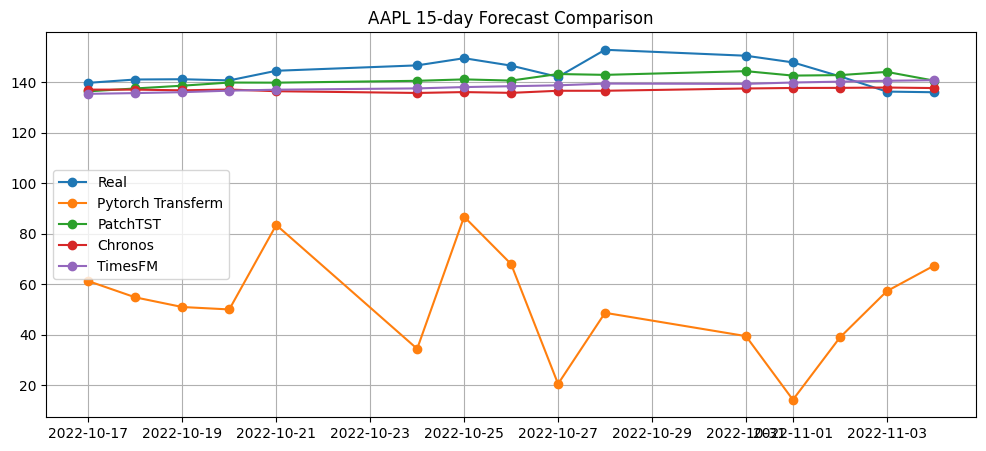
畫圖

plt.figure(figsize=(12,5))


plt.plot(
    future_date,
    real_price,
    marker="o",
    label="Real"
)


plt.plot(
    future_date,
    stock_pred_price,
    marker="o",
    label="Pytorch Transferm"
)

plt.plot(
    future_date,
    patch_price,
    marker="o",
    label="PatchTST"
)


plt.plot(
    future_date,
    chronos_price,
    marker="o",
    label="Chronos"
)


plt.plot(
    future_date,
    timesfm_price,
    marker="o",
    label="TimesFM"
)


plt.title(
    "AAPL 15-day Forecast Comparison"
)


plt.legend()
plt.grid()

plt.show()

from sklearn.metrics import root_mean_squared_error
print("Pytorch Transformer RMSE:",root_mean_squared_error(real_price,stock_pred_price))
print("PatchTST RMSE:",root_mean_squared_error(real_price,patch_price))
print("Chronos RMSE:",root_mean_squared_error(real_price,chronos_price))
print("TimesFM RMSE:",root_mean_squared_error(real_price,timesfm_price))

Pytorch Transformer RMSE: 94.45434107394114
PatchTST RMSE: 5.4334922412162365
Chronos RMSE: 8.667400348849727
TimesFM RMSE: 7.529667051063065